Finding all places within a country boundary sounds simple — just use ST_Contains or ST_Within, right? In practice, country polygons are incredibly detailed, and that detail kills query performance.

I expected polygon simplification to be a silver bullet. Simplify the geometry, reduce vertices, speed everything up. The data told a different story: simplification made things slower for 53% of the 200 divisions I tested. But for the right polygons — complex coastlines with moderate place counts — it delivered 37x speedups.

Here's what I learned benchmarking twelve approaches across 60 million places.

The Setup

I'm using the Overture Maps dataset loaded into PostgreSQL with PostGIS. All code and benchmark queries are in the overturemaps-pg repo.

git clone https://github.com/nikmarch/overturemaps-pg
cd overturemaps-pg
./start.sh divisions places

This spins up a PostgreSQL + PostGIS instance in Docker and imports ~60 million places and all division boundaries.

The Problem

My first attempt used PostGIS geography type for global accuracy:

EXPLAIN ANALYZE
SELECT * FROM places p
JOIN divisions d ON ST_Covers(d.geography, p.geography)
WHERE d.id = '6aaadea0-9c48-4af0-a47f-bbe020540580';  -- Argentina

After 16 hours, the query was still running. Two factors make this painfully slow:

Geography vs Geometry — The geography type calculates on a spheroid (mathematically correct but expensive). For point-in-polygon checks across millions of rows, the accuracy gain over planar geometry is negligible, but the cost is massive.

Type Calculations Use Case
geography Spheroidal (accurate, slow) Small areas, precise distances
geometry Planar (fast, approximate) Large datasets, containment checks

Polygon Complexity — Country boundaries in Overture Maps are highly detailed. Argentina's Patagonian coastline has 200,000+ vertices. Every ST_Covers check must test against all of them.

The config query selects the top 200 divisions by area with >1,000 vertices — these are our benchmark candidates:

-- Top 20 most complex division geometries (from 200 benchmarked)
SELECT name, osm_id, class, points, round(area, 1) AS area
FROM 'https://raw.githubusercontent.com/nikmarch/overturemaps-pg/master/pages/optimizing-spatial-queries/queries/_config.csv'
ORDER BY area DESC
LIMIT 20;

Note: Some divisions have multiple geometries (land borders vs maritime boundaries), which is why you'll see the same osm_id appear more than once. I benchmarked both to see if one is consistently faster — it would be interesting to find out whether the maritime boundary can be used instead of the land one.

The Optimization Journey

Each step here follows from the previous — every idea is a reaction to what didn't work or could be better.

JOIN — The naive approach after switching to geometry: just ST_Covers, no tricks.

+ bbox — I didn't come up with this one. While writing the benchmark queries, the AI assistant silently added a && bounding box pre-filter. I had never considered using it, but decided to test it anyway to see if it actually matters.

WHERE p.geometry && div.geom          -- fast: uses spatial index
  AND ST_Covers(div.geom, p.geometry) -- slow: only runs on candidates

CTE — The join re-evaluates the division lookup for every row. Extract it into a CTE so the geometry is fetched once.

CTE MATERIALIZED — PostgreSQL might inline the CTE and re-evaluate it anyway. Force it to materialize with MATERIALIZED.

Simplify + buffer — The polygon itself is the bottleneck — 200K+ vertices per ST_Covers call. Use ST_Simplify to reduce complexity, but simplification can cut inside the original boundary and miss places near the border. Fix: simplify, then buffer outward to ensure the result fully contains the original.

Since geometry operates in degrees, we convert meters: 1000 / 111320 ≈ 0.009 for ~1km (1 degree ≈ 111,320m at the equator).

ST_Buffer(ST_Simplify(geometry, 0.01), 0.01)  -- ~1.1km tolerance & buffer

Chile's coastline with original and simplified polygon layers overlaid — the buffered versions fully contain the original boundary

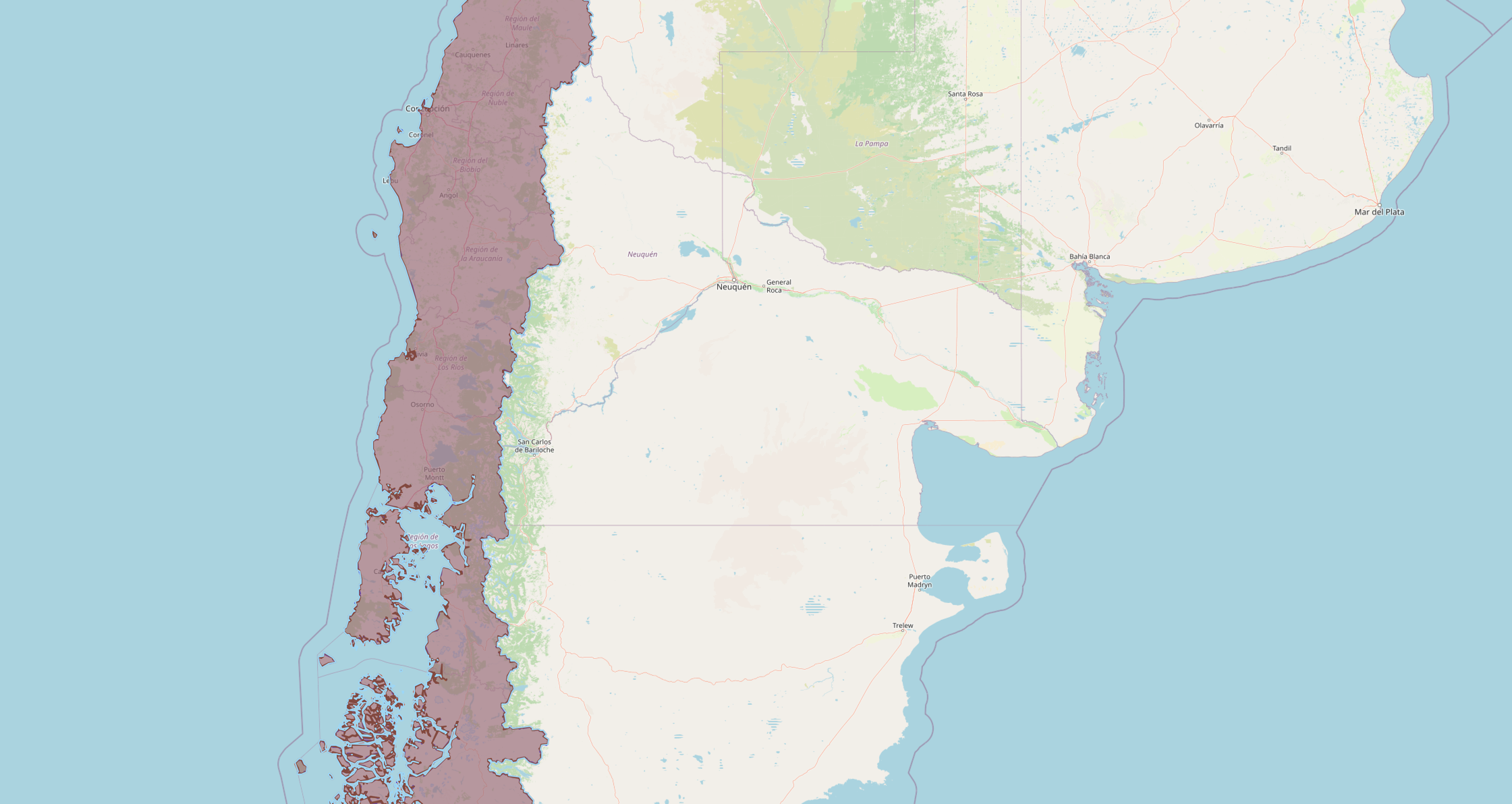
Chile's Patagonian coastline: the original polygon (207K vertices) with simplified and buffered variants overlaid. The buffer ensures no places near the border are missed.

Preserve topologyST_Simplify uses Douglas-Peucker, which can produce self-intersecting polygons. ST_SimplifyPreserveTopology avoids this.

Preserve topology + buffer — Combine topology-safe simplification with a safety buffer to guarantee no misses.

Every approach above is benchmarked with and without the && bbox pre-filter, so you can see its impact at each level of optimization.

The Benchmark

I automated all twelve approaches across 200 divisions. The database is restarted between approaches to ensure cold cache. Each query is in its own SQL file:

# Approach bbox Idea
01 JOIN Naive baseline
02 JOIN && Add spatial index pre-filter
03 CTE Extract division lookup
04 CTE &&
05 CTE MATERIALIZED Force single evaluation
06 CTE MATERIALIZED &&
07 Simplified + buffer Reduce vertices
08 Simplified + buffer &&
09 Preserve topology Topology-safe, no buffer
10 Preserve topology &&
11 Topology + buffer Topology-safe + buffer
12 Topology + buffer &&

Results

The benchmark results are published as a CSV. Click Run to query them with DuckDB right in your browser.

The Overall Picture

First, here's the aggregate view — average timings across all 200 divisions:

-- Timing percentiles per approach across 200 divisions (ms)
WITH r AS (
    SELECT * FROM 'https://raw.githubusercontent.com/nikmarch/overturemaps-pg/master/pages/optimizing-spatial-queries/results/results_2026-02-07_052445.csv'
)
SELECT '01_join' AS approach,
    round(avg("01_join_total_time"), 0) AS avg,
    round(quantile_cont("01_join_total_time", 0.50), 0) AS p50,
    round(quantile_cont("01_join_total_time", 0.95), 0) AS p95,
    round(quantile_cont("01_join_total_time", 0.99), 0) AS p99,
    round(min("01_join_total_time"), 0) AS min,
    round(max("01_join_total_time"), 0) AS max FROM r
UNION ALL
SELECT '02_join_bbox',
    round(avg("02_join_bbox_total_time"), 0),
    round(quantile_cont("02_join_bbox_total_time", 0.50), 0),
    round(quantile_cont("02_join_bbox_total_time", 0.95), 0),
    round(quantile_cont("02_join_bbox_total_time", 0.99), 0),
    round(min("02_join_bbox_total_time"), 0),
    round(max("02_join_bbox_total_time"), 0) FROM r
UNION ALL
SELECT '03_cte',
    round(avg("03_cte_total_time"), 0),
    round(quantile_cont("03_cte_total_time", 0.50), 0),
    round(quantile_cont("03_cte_total_time", 0.95), 0),
    round(quantile_cont("03_cte_total_time", 0.99), 0),
    round(min("03_cte_total_time"), 0),
    round(max("03_cte_total_time"), 0) FROM r
UNION ALL
SELECT '04_cte_bbox',
    round(avg("04_cte_bbox_total_time"), 0),
    round(quantile_cont("04_cte_bbox_total_time", 0.50), 0),
    round(quantile_cont("04_cte_bbox_total_time", 0.95), 0),
    round(quantile_cont("04_cte_bbox_total_time", 0.99), 0),
    round(min("04_cte_bbox_total_time"), 0),
    round(max("04_cte_bbox_total_time"), 0) FROM r
UNION ALL
SELECT '05_cte_mat',
    round(avg("05_cte_materialized_total_time"), 0),
    round(quantile_cont("05_cte_materialized_total_time", 0.50), 0),
    round(quantile_cont("05_cte_materialized_total_time", 0.95), 0),
    round(quantile_cont("05_cte_materialized_total_time", 0.99), 0),
    round(min("05_cte_materialized_total_time"), 0),
    round(max("05_cte_materialized_total_time"), 0) FROM r
UNION ALL
SELECT '06_cte_mat_bbox',
    round(avg("06_cte_materialized_bbox_total_time"), 0),
    round(quantile_cont("06_cte_materialized_bbox_total_time", 0.50), 0),
    round(quantile_cont("06_cte_materialized_bbox_total_time", 0.95), 0),
    round(quantile_cont("06_cte_materialized_bbox_total_time", 0.99), 0),
    round(min("06_cte_materialized_bbox_total_time"), 0),
    round(max("06_cte_materialized_bbox_total_time"), 0) FROM r
UNION ALL
SELECT '07_simplified',
    round(avg("07_simplified_total_time"), 0),
    round(quantile_cont("07_simplified_total_time", 0.50), 0),
    round(quantile_cont("07_simplified_total_time", 0.95), 0),
    round(quantile_cont("07_simplified_total_time", 0.99), 0),
    round(min("07_simplified_total_time"), 0),
    round(max("07_simplified_total_time"), 0) FROM r
UNION ALL
SELECT '08_simplified_bbox',
    round(avg("08_simplified_bbox_total_time"), 0),
    round(quantile_cont("08_simplified_bbox_total_time", 0.50), 0),
    round(quantile_cont("08_simplified_bbox_total_time", 0.95), 0),
    round(quantile_cont("08_simplified_bbox_total_time", 0.99), 0),
    round(min("08_simplified_bbox_total_time"), 0),
    round(max("08_simplified_bbox_total_time"), 0) FROM r
UNION ALL
SELECT '09_topo',
    round(avg("09_simplified_preserve_topology_total_time"), 0),
    round(quantile_cont("09_simplified_preserve_topology_total_time", 0.50), 0),
    round(quantile_cont("09_simplified_preserve_topology_total_time", 0.95), 0),
    round(quantile_cont("09_simplified_preserve_topology_total_time", 0.99), 0),
    round(min("09_simplified_preserve_topology_total_time"), 0),
    round(max("09_simplified_preserve_topology_total_time"), 0) FROM r
UNION ALL
SELECT '10_topo_bbox',
    round(avg("10_simplified_preserve_topology_bbox_total_time"), 0),
    round(quantile_cont("10_simplified_preserve_topology_bbox_total_time", 0.50), 0),
    round(quantile_cont("10_simplified_preserve_topology_bbox_total_time", 0.95), 0),
    round(quantile_cont("10_simplified_preserve_topology_bbox_total_time", 0.99), 0),
    round(min("10_simplified_preserve_topology_bbox_total_time"), 0),
    round(max("10_simplified_preserve_topology_bbox_total_time"), 0) FROM r
UNION ALL
SELECT '11_topo_buf',
    round(avg("11_simplified_preserve_topology_buffered_total_time"), 0),
    round(quantile_cont("11_simplified_preserve_topology_buffered_total_time", 0.50), 0),
    round(quantile_cont("11_simplified_preserve_topology_buffered_total_time", 0.95), 0),
    round(quantile_cont("11_simplified_preserve_topology_buffered_total_time", 0.99), 0),
    round(min("11_simplified_preserve_topology_buffered_total_time"), 0),
    round(max("11_simplified_preserve_topology_buffered_total_time"), 0) FROM r
UNION ALL
SELECT '12_topo_buf_bbox',
    round(avg("12_simplified_preserve_topology_buffered_bbox_total_time"), 0),
    round(quantile_cont("12_simplified_preserve_topology_buffered_bbox_total_time", 0.50), 0),
    round(quantile_cont("12_simplified_preserve_topology_buffered_bbox_total_time", 0.95), 0),
    round(quantile_cont("12_simplified_preserve_topology_buffered_bbox_total_time", 0.99), 0),
    round(min("12_simplified_preserve_topology_buffered_bbox_total_time"), 0),
    round(max("12_simplified_preserve_topology_buffered_bbox_total_time"), 0) FROM r
ORDER BY avg DESC;

The averages look close. That's because simplification's impact varies wildly by division. Averages hide the real story.

The Real Story: It Depends

Let's classify each division — did simplification actually help?

-- Classify divisions: where does simplified help?
SELECT
    CASE
        WHEN "01_join_total_time" / "07_simplified_total_time" > 1.1 THEN 'simplified faster'
        WHEN "01_join_total_time" / "07_simplified_total_time" < 0.9 THEN 'simplified slower'
        ELSE 'similar'
    END AS result,
    count(*) AS divisions,
    round(100.0 * count(*) / sum(count(*)) OVER (), 1) AS pct
FROM 'https://raw.githubusercontent.com/nikmarch/overturemaps-pg/master/pages/optimizing-spatial-queries/results/results_2026-02-07_052445.csv'
GROUP BY 1
ORDER BY divisions DESC;

The majority of divisions are slower with simplification. That was not what I expected.

Where Simplification Shines

The wins are concentrated in divisions with complex coastlines and moderate place counts. Chile, Argentina, Tanzania, South Africa — countries where the original polygon has tens or hundreds of thousands of vertices tracing intricate coastlines:

-- Top 15 where simplified wins (highest speedup)
SELECT name, points,
    split_part("01_join_total", chr(10), 3)::int AS join_count,
    split_part("07_simplified_total", chr(10), 3)::int AS simplified_count,
    round("01_join_total_time", 0) AS join_ms,
    round("07_simplified_total_time", 0) AS simplified_ms,
    round("01_join_total_time" / "07_simplified_total_time", 1) AS speedup
FROM 'https://raw.githubusercontent.com/nikmarch/overturemaps-pg/master/pages/optimizing-spatial-queries/results/results_2026-02-07_052445.csv'
WHERE "07_simplified_total_time" > 0
ORDER BY "01_join_total_time" / "07_simplified_total_time" DESC
LIMIT 15;

These are the headline numbers — 37x for Tanzania, 31x for Chile, 30x for Argentina. When you have 170,000 vertices and the simplified polygon drops that to a few hundred, the ST_Covers savings are enormous. Notice the simplified count is always equal or higher — the buffer guarantees no places are missed. For full accuracy you could run the exact join as a second pass on the simplified result set, but I decided the marginal extras weren't worth doubling the query time.

Tanzania's coastline with original and simplified polygon layers — the simplified boundary cuts through inlets while the buffer expands to cover them

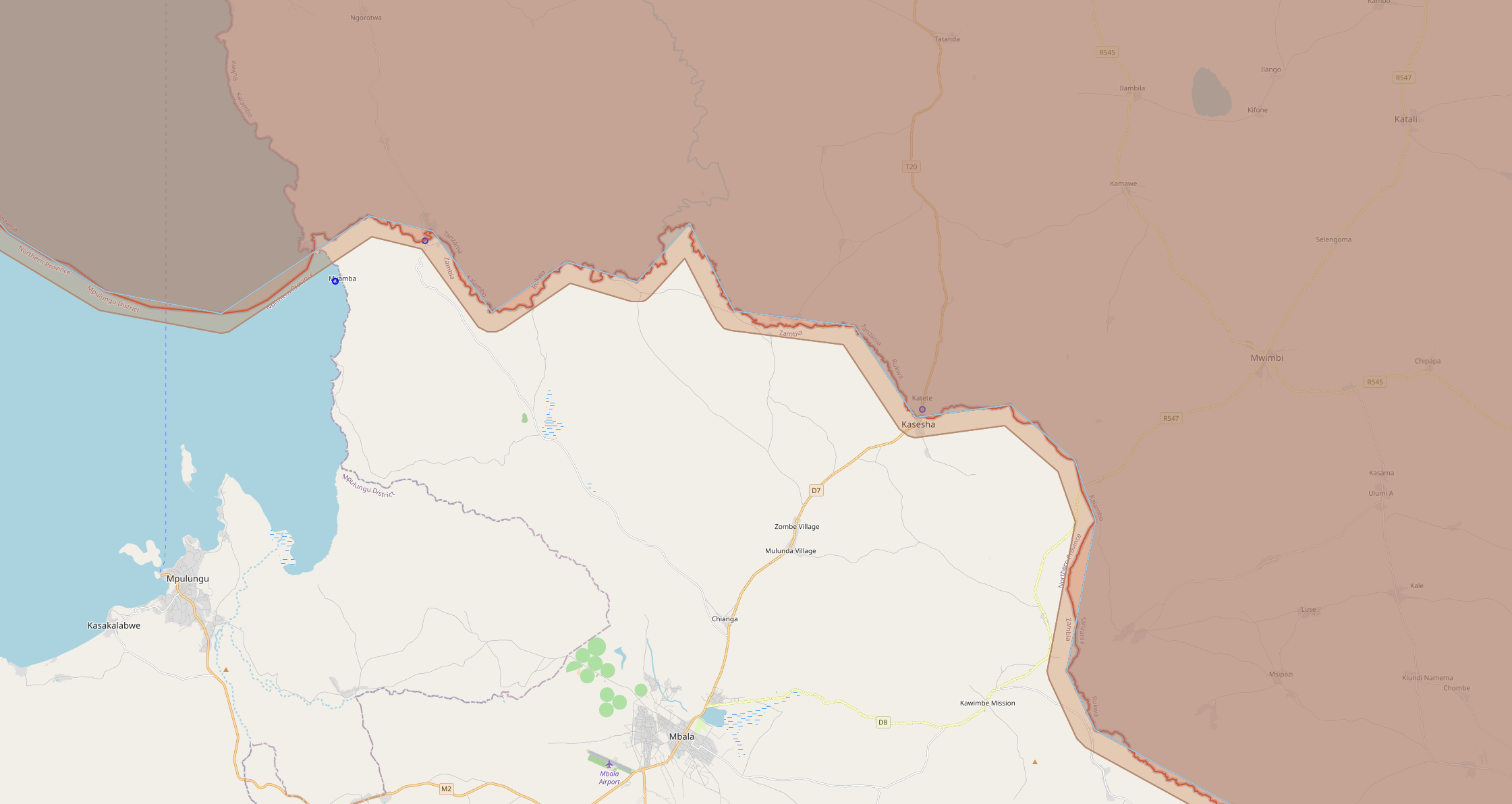
Tanzania's coastline: the blue original boundary traces every inlet, while the simplified layers smooth it out. The buffer (outer edge) ensures full coverage.

Where Simplification Hurts

Now the other side. The divisions where simplification made things worse:

-- Top 15 where simplified hurts (highest slowdown)
SELECT name, points,
    split_part("01_join_total", chr(10), 3)::int AS join_count,
    split_part("07_simplified_total", chr(10), 3)::int AS simplified_count,
    round("01_join_total_time", 0) AS join_ms,
    round("07_simplified_total_time", 0) AS simplified_ms,
    round("07_simplified_total_time" / "01_join_total_time", 1) AS slowdown
FROM 'https://raw.githubusercontent.com/nikmarch/overturemaps-pg/master/pages/optimizing-spatial-queries/results/results_2026-02-07_052445.csv'
WHERE "01_join_total_time" > 0
ORDER BY "07_simplified_total_time" / "01_join_total_time" DESC
LIMIT 15;

The pattern: large countries with millions of places (US, Russia, China, India) or tiny Arctic regions where the overhead isn't worth it.

Speedup by Complexity Bucket

Breaking results down by polygon complexity shows the pattern more clearly:

-- Speedup by polygon complexity: p50 per approach (ms)
SELECT
    CASE
        WHEN points >= 100000 THEN '100k+'
        WHEN points >= 50000 THEN '50k-100k'
        WHEN points >= 10000 THEN '10k-50k'
        ELSE '<10k'
    END AS complexity,
    count(*) AS n,
    round(quantile_cont("01_join_total_time", 0.50), 0) AS "join",
    round(quantile_cont("03_cte_total_time", 0.50), 0) AS cte,
    round(quantile_cont("05_cte_materialized_total_time", 0.50), 0) AS cte_mat,
    round(quantile_cont("07_simplified_total_time", 0.50), 0) AS simplified,
    round(quantile_cont("09_simplified_preserve_topology_total_time", 0.50), 0) AS topo,
    round(quantile_cont("11_simplified_preserve_topology_buffered_total_time", 0.50), 0) AS topo_buf,
    round(quantile_cont("01_join_total_time", 0.50) / quantile_cont("07_simplified_total_time", 0.50), 1) AS speedup,
FROM 'https://raw.githubusercontent.com/nikmarch/overturemaps-pg/master/pages/optimizing-spatial-queries/results/results_2026-02-07_052445.csv'
GROUP BY 1
ORDER BY "join" DESC;

Individual Division Results

-- Top 20 divisions by polygon complexity with all approaches (ms)
SELECT
    name, points,
    round("01_join_total_time", 0) AS "join",
    round("03_cte_total_time", 0) AS cte,
    round("05_cte_materialized_total_time", 0) AS cte_mat,
    round("07_simplified_total_time", 0) AS simplified,
    round("09_simplified_preserve_topology_total_time", 0) AS topo,
    round("11_simplified_preserve_topology_buffered_total_time", 0) AS topo_buf,
    round("01_join_total_time" / "07_simplified_total_time", 1) AS speedup,
FROM 'https://raw.githubusercontent.com/nikmarch/overturemaps-pg/master/pages/optimizing-spatial-queries/results/results_2026-02-07_052445.csv'
ORDER BY points DESC
LIMIT 20;

Accuracy Check

Which approach finds the same places as the baseline join? The ideal approach finds the same places (no misses, minimal extras from buffer expansion) while being the fastest:

-- Pick the winner: accuracy vs speed across all divisions
WITH r AS (
    SELECT *,
        split_part("01_join_total", chr(10), 3)::int AS j,
        split_part("03_cte_total", chr(10), 3)::int AS c,
        split_part("05_cte_materialized_total", chr(10), 3)::int AS cm,
        split_part("07_simplified_total", chr(10), 3)::int AS s,
        split_part("09_simplified_preserve_topology_total", chr(10), 3)::int AS t,
        split_part("11_simplified_preserve_topology_buffered_total", chr(10), 3)::int AS tb,
    FROM 'https://raw.githubusercontent.com/nikmarch/overturemaps-pg/master/pages/optimizing-spatial-queries/results/results_2026-02-07_052445.csv'
    WHERE "01_join_total" IS NOT NULL
),
stats AS (
    SELECT '01_join' AS approach, sum(j) AS places,
        count(*) FILTER (WHERE j < j) AS fewer,
        count(*) FILTER (WHERE j > j) AS more,
        round(sum("01_join_total_time"), 0) AS total_ms FROM r
    UNION ALL
    SELECT '03_cte', sum(c),
        count(*) FILTER (WHERE c < j) AS fewer,
        count(*) FILTER (WHERE c > j) AS more,
        round(sum("03_cte_total_time"), 0) FROM r
    UNION ALL
    SELECT '05_cte_mat', sum(cm),
        count(*) FILTER (WHERE cm < j),
        count(*) FILTER (WHERE cm > j),
        round(sum("05_cte_materialized_total_time"), 0) FROM r
    UNION ALL
    SELECT '07_simplified', sum(s),
        count(*) FILTER (WHERE s < j),
        count(*) FILTER (WHERE s > j),
        round(sum("07_simplified_total_time"), 0) FROM r
    UNION ALL
    SELECT '09_topo', sum(t),
        count(*) FILTER (WHERE t < j),
        count(*) FILTER (WHERE t > j),
        round(sum("09_simplified_preserve_topology_total_time"), 0) FROM r
    UNION ALL
    SELECT '11_topo_buf', sum(tb),
        count(*) FILTER (WHERE tb < j),
        count(*) FILTER (WHERE tb > j),
        round(sum("11_simplified_preserve_topology_buffered_total_time"), 0) FROM r
)
SELECT
    s.approach,
    s.places,
    s.places - b.places AS count_diff,
    s.fewer AS divisions_fewer,
    s.more AS divisions_more,
    s.total_ms,
    round(b.total_ms::float / s.total_ms, 1) AS speedup,
FROM stats s, (SELECT * FROM stats WHERE approach = '01_join') b
ORDER BY s.total_ms;

The CSV also contains full EXPLAIN ANALYZE output for every query:

-- EXPLAIN ANALYZE plans for United States (land boundary)
SELECT
    replace("01_join_analyze", '\n', chr(10)) AS query_plan,
FROM 'https://raw.githubusercontent.com/nikmarch/overturemaps-pg/master/pages/optimizing-spatial-queries/results/results_2026-02-07_052445.csv'
WHERE name = 'United States' AND class = 'land';

Why Simplification Can Be Slower

The results surprised me, so I dug into why simplification hurts for large countries.

The buffer expands the polygon. ST_Buffer(ST_Simplify(geom, 0.01), 0.01) simplifies the boundary but also pushes it ~1km outward in every direction. For a country like the United States, this expanded polygon matches more places in the spatial index — places that weren't within the original boundary.

More matches = more I/O. For divisions with millions of places (the US has ~10M, Russia ~2M, China ~8M), the extra rows from buffer expansion cost more to scan than the vertex reduction saves. The simplification trades CPU savings (fewer vertices per ST_Covers call) for I/O costs (more rows to check).

Small divisions: overhead isn't worth it. For tiny Arctic regions or island nations with few places, the ST_Simplify + ST_Buffer computation itself adds overhead that exceeds any vertex-check savings.

The sweet spot: moderate place count + complex coastline. Chile has 170K+ vertices tracing its 6,000km coastline but only ~500K places. Simplification slashes the vertex count while the buffer expansion adds minimal extra rows. That's why Chile sees a 31x speedup while the US sees a 5x slowdown.

Tradeoffs

Conclusion

  1. Use geometry, not geography for large-scale containment queries — this is universally true and the biggest single improvement.
  2. Profile before simplifying — simplification's impact depends on polygon shape and place density, not just vertex count.
  3. Complex coastlines with moderate place counts benefit most — Tanzania (37x), Chile (31x), Argentina (30x). If a polygon has many vertices tracing an intricate coastline and a manageable number of places, simplification is a big win.
  4. For large countries with millions of places, plain joins are hard to beat — the buffer expansion adds more I/O than the vertex reduction saves.

There's no universal "fastest approach." The right optimization depends on your data. Benchmark your actual workload.


Tested with PostgreSQL 16 and PostGIS 3.4 using the Overture Maps dataset. Full benchmark code: github.com/nikmarch/overturemaps-pg